Signal Plots

The Signal Plot Editor is a powerful tool for creating and managing time-based sequences of actions. These actions, called Control Points, can manipulate Modbus coils and registers, call system methods, and control PID loops. This allows for the automation of complex, multi-step processes with precise timing.

The Signal Plot Editor Interface

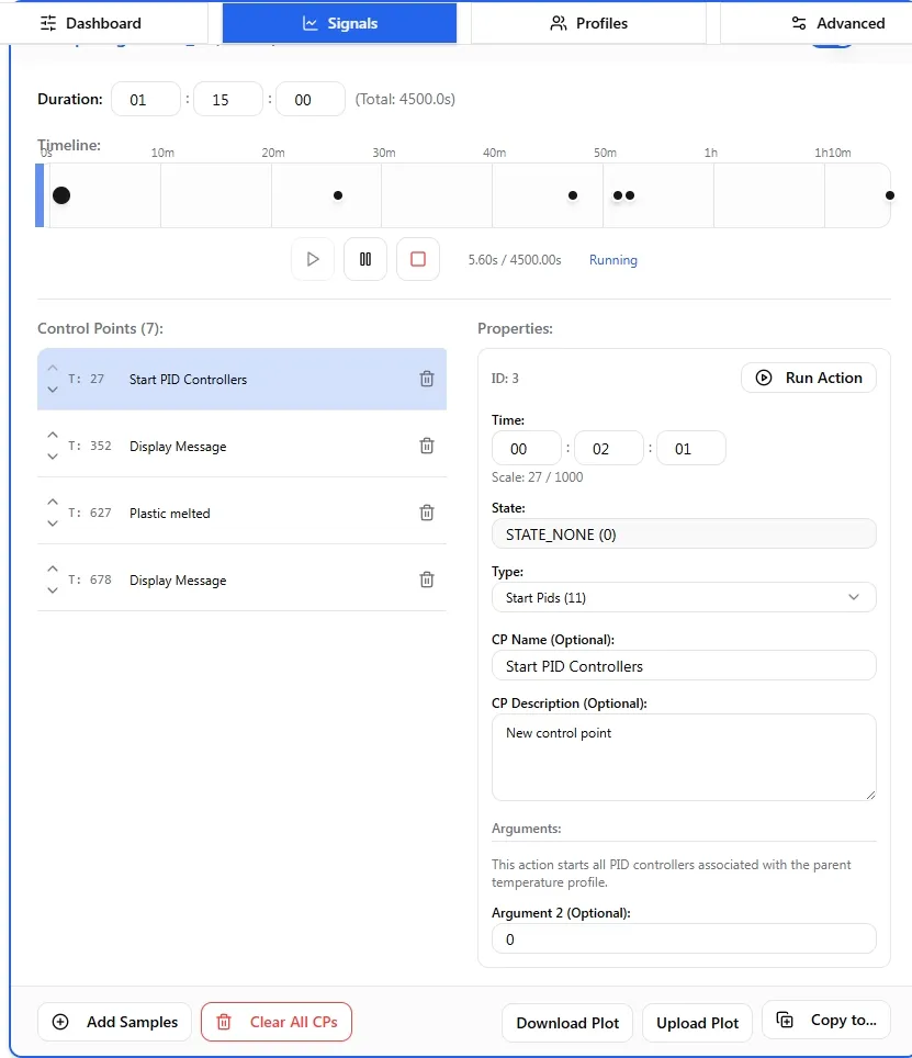
The editor is organized into cards, with each card representing a single Signal Plot. Here’s a breakdown of the main components:

Global Controls

At the top of the page, you’ll find global controls for managing all your plots at once:

• Download All JSON: Exports all currently configured signal plots into a single JSON file. This is highly recommended for backing up your configurations.
• Upload All JSON: Imports a previously saved JSON file to restore or deploy a full set of signal plots. This will overwrite all existing plots.

The Plot Card

Each plot is managed through its own card, which contains all the tools needed to configure its behavior.

1. Plot Header

The header provides identifying information and the primary enable/disable control for the plot.

• Plot Name: A user-friendly name for the plot (e.g., “Heating Cycle”, “Extrusion Profile”). Click the name to edit it. Give your plots descriptive names!
• Slot: A unique ID number for the plot. This is how the system identifies the plot internally.
• Enable Switch: A toggle switch on the right. A plot must be enabled for its control points to be executed by the system. You can prepare complex plots and leave them disabled until they are needed.

2. Duration

This setting defines the total running time for the plot. Note: When a Signal Plot is used as part of a larger Temperature Profile, this duration is typically inherited from the parent profile’s settings and may not be editable here.

• TimeCode Editor: In standalone mode, you can set the duration in HH:MM:SS.ms format.
• The duration is the canvas on which you place your control points. A control point’s execution time is relative to this total duration. If you change the duration, the actual execution time of all control points will scale accordingly.

3. Timeline

The timeline is the visual core of the editor, showing your control points laid out over the plot’s duration.

• Adding Control Points: Double-click anywhere on the timeline to add a new control point at that position.
• Moving Control Points: Click and drag a control point marker left or right to adjust its timing.
• Selecting Control Points: Simply click a control point marker. This will highlight it and display its details in the Properties pane.
• Playback Head: The vertical red line indicates the current progress of the plot when it’s running. When paused, you can drag the playback head to scrub through the timeline and manually set the execution time.

4. Playback Controls (First Plot Only)

These controls are available only on the first plot in the list and control its execution.

• Play/Resume: Starts the plot from the beginning or resumes it if paused.
• Pause: Halts the plot at its current position.
• Stop: Stops the plot and resets its elapsed time to zero.

5. Control Points & Properties

This section is a split view for managing the fine details of your control points.

• Control Points List: A list of all control points in the plot, sorted by time. This is a great way to see all your steps in order. You can select, re-order, and delete CPs from this list.
• Properties Pane: When a control point is selected (either from the timeline or the list), its properties are displayed here. You can configure its name, type, and arguments. See the Control Point Types section below for details.

6. Plot Footer & Actions

The footer contains tools for saving, reverting, and managing the control points within the plot.

• Save Changes / Revert: When you modify a plot, it becomes “dirty,” and these buttons will appear.
  • Save Changes: Saves the current state of the plot (name, duration, CPs) to the controller.
  • Revert: Discards all changes made since the last save.
• Add Samples: Adds a pre-configured set of sample control points to the timeline. This is useful for testing or as a template.
• Clear All CPs: Deletes all control points from the plot.
• Download Plot / Upload Plot: Similar to the global controls, but for a single plot only. This allows you to share or back up individual sequences.

Control Point Types

Control Points are the individual actions that make up a signal plot. Each has a specific Type that determines what it does, and a set of Arguments to configure its behavior.

MB_WRITE_COIL

This is one of the most common types. It changes the state of a single Modbus coil (a digital output).

• Purpose: To turn something ON or OFF.
• Arguments:
  • arg_0 (Coil Address): The address of the Modbus coil to write to. You can type an address or select from a list of known coils.
  • arg_1 (Coil Value): The state to set the coil to. This is represented as a toggle switch: ON corresponds to a value of 1, and OFF corresponds to a value of 0.

MB_WRITE_HOLDING_REGISTER

This type writes a numeric value to a single Modbus holding register.

• Purpose: To set a parameter, like a target speed, temperature, or position.
• Arguments:
  • arg_0 (Register Address): The address of the Modbus holding register to write to. You can type an address or select from a list of known registers.
  • arg_1 (Register Value): The numeric value to write into the register.

CALL_METHOD

This is an advanced type that allows a plot to execute a pre-registered function on the system’s backend.

• Purpose: To trigger complex, non-Modbus actions that have been exposed as callable methods.
• Arguments:
  • arg_0 (Method ID): The unique ID of the registered method to call.
  • arg_1 (Argument 1): A numeric value to pass as an argument to the method.

START_PIDS

This action is specifically related to temperature control profiles.

• Purpose: To enable all PID controllers associated with the parent temperature profile. This effectively “turns on” active temperature regulation.
• Arguments: None.

STOP_PIDS

This action is the counterpart to START_PIDS.

• Purpose: To disable all PID controllers associated with the parent temperature profile. This “turns off” active temperature regulation.
• Arguments: None.

PAUSE_PROFILE

This action pauses the execution of the parent profile.

• Purpose: To halt the process temporarily, perhaps to wait for a manual inspection or external event. The profile can be resumed later.
• Arguments: None.

Recommendations & Best Practices

• PID Control Strategy: For any process involving heating, it’s crucial to manage your PID controllers effectively.

  • Best Practice: Place a START_PIDS control point near the beginning of your plot (e.g., at time 0 or shortly after) and a STOP_PIDS control point near the end. This ensures that the heaters are actively managed during your process but are safely turned off when the process is complete.

• Descriptive Naming: As plots become more complex, good names are essential.

  • Name your plots: Plastic A - 220C Extrusion is much better than Plot 3.
  • Name your control points: Use the optional “CP Name” field in the properties. Turn on conveyor belt is clearer than a MB_WRITE_COIL point with address 105.

• Save Your Work: The editor does not auto-save. A plot with a blue border is “dirty” and has unsaved changes. Always remember to click Save Changes for each plot you edit.

• Backup with JSON: Before a major reconfiguration, use the Download All JSON button to create a backup. If something goes wrong, you can easily restore your previous working state.

• Use the Timeline and List Together: The timeline is great for a high-level view and rough timing adjustments. The Control Points list is excellent for reviewing the exact sequence of events and making precise selections.